Adding or correcting data-points with Linear Prediction
The expression "Linear Prediction" identifies a principle and a technique which, although not essential for NMR, can be extremely useful in particular cases. The principle is that, just because the FID is the sum of regular (sinusoidal) waves, it is possible to extrapolate a fragment of a FID to reconstruct the whole or to prolong it forward and/or backward. LP can also be used to calculate the parameters (e.g. frequencies and intensities of all signals) that describe a spectrum. (iNMR does not implement this feature). FT has the advantage, over LP, of being much faster and stable and of being of more general applicability.
Normally you don't need to know anything about LP. If you want to use it as an alternative to zero-filling, it is enough to check the LP option inside the FT dialog. iNMR automatically sets all the parameters for you.
In rare cases you may want to use the “Linear Prediction” command. Its flexibility allows you to perform back- or forward prediction, to reconstruct portions of the FID (or interferogram in nD spectroscopy), to give an hint about the number of peaks contained into the spectrum. You can repeat LP how many times you want, yet only the final values are stored into the document. iNMR allows you to perform up to three LP runs with a single operations. Thanks to this mechanism, up to three runs per dimensions can be stored into each document. You must furnish the following parameters:
- Limits for the interval to be corrected or generated. You specify the position in time domain, where the unit is the dwell time (each couple of sampled point). This is the same unit called “point” by iNMR. The first point usually has an index of zero, with the notable exception of digitally filtered Bruker spectra, where the FID starts from negative values.
- Number of experimental points which represent the raw material on which to build the LP. Normally you specify all the points in the spectrum. If you specify an higher number, iNMR will reduce it to the maximum possible value.
- The number of coefficients. Ideally you should guess the exact number of peaks in the transformed spectrum. The outcome of LP depends on the correct choice of this value. Sometimes specifying a little more or a little less peaks can generate intolerable noise and artifacts. Regarding the choice of this parameter, there are a few known rules: the first rule is that the higher the value, the longer the time that LP requires; the second rule is to avoid the “Fast LP” when the numbe of coefficients is > 24, because it's the less stable algorithm. The other algorithms are able to ignore this value, if they detect that the spectrum contains less peaks than those declared by you.
The stand-alone LP and the LP-filling, even when using the same algorithms, are not equivalent. When used in 2D (phase-sensitive) spectroscopy, stand-alone LP comes before shuffling (data-reduction), while LP-filling comes after. It's unlikely, yet possible, that the outcomes are different.
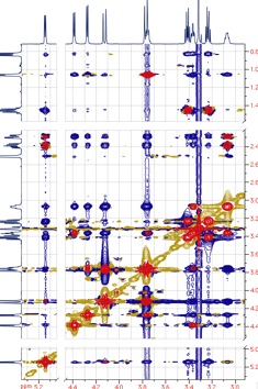
It is also important which phase-sensitive scheme is adopted. If the next FT is a real FT (when the TPPI scheme is in use), the Fast LP creates a counter-diagonal. In the other cases (Ruben-States and States-TPPI), signals near the diagonal are marred by noise produced by the LP. In most cases this is preferable to the counter-diagonal.
Algorithms
You can choose among 3 different algorithms to compute the LP coefficients. Singular Value Decomposition is probably the best compromise between speed and stability. Our implementation is optimized for today's CPUs. LP-filling follows the Fast algorithm by Cybenko, which is less stable. It has been optimized for the old G3 processor. The Zhu and Bax method is stable, but only for forward prediction.
See also