So You Want to Be a Phase-Correction Wizard?

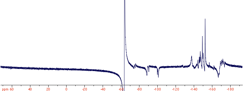
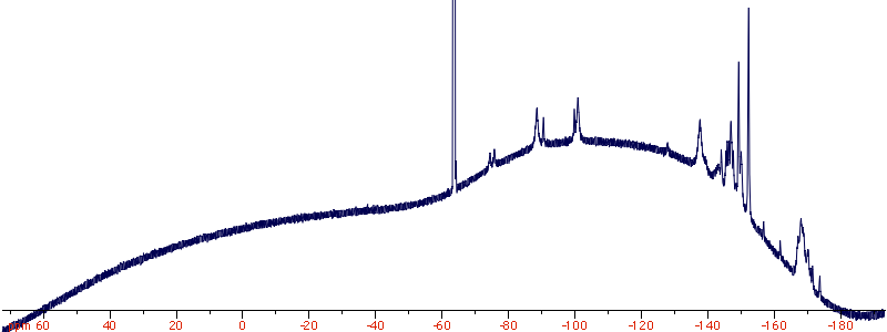
From an instrumental point of view, the main difference between a generic proton spectrum and the spectrum of another nucleus is that, in the latter case, the spectral width is much larger. Correcting the phase and the baseline can become more difficult than usual. The solution seems more difficult to find in the case of Varian spectra, although these spectra are not worse than those acquired with other brands of spectrometer. After following this short tutorial, whichever spectrometer you have, you'll have learned (or re-learned) a couple of useful rules. We are going to show two simple and alternative solutions, both valid and both simple. We'll be working on a real case ¹⁹F spectrum you can download from here. The spectrum, before any phase or baseline correction, is hown into the first picture:

A Quick Solution

The phase correction stage is where people usually end trapped into. In all the cases I have met so far, the solution was readily available, because the right correction had already been found by the spectrometer and saved into the original files. With TextEdit (or any other text editor) open the “procpar” file and look for “lp” (the Varian name for first order phase correction). You will find several occurrences, including the description of the parameter:

lp 1 1 3600 -3600 0.1 4 1 3 1 64
1 -1049.58420782 
0 

The value is: -1049.58420782. iNMR follows the inverse convention for the sign, so our starting value for the first order phase correction inside iNMR will be 1050. Now it is relatively easy to find the zero-order correction. My preference goes for the following combination:
zero order correction = -154
first order corr. = 1073
The large first-order correction has an unfortunate effect on the baseline:

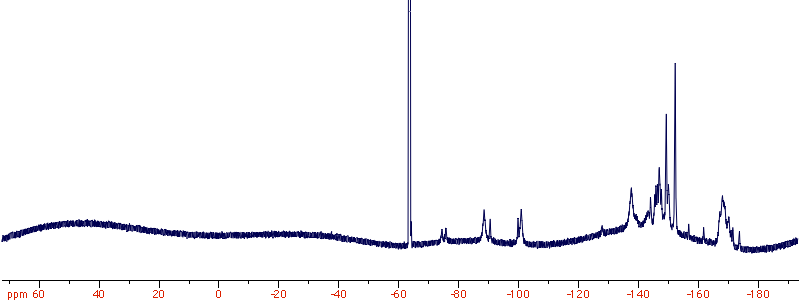
The latter is then corrected with the following parameters:

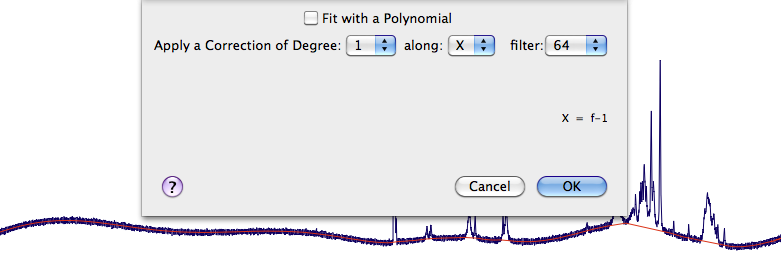
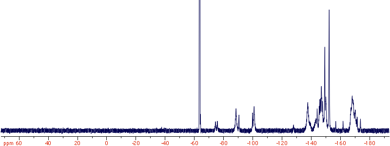
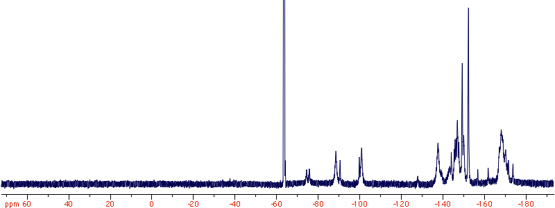
You can easily verify that, in this particular case, the critical parameter is the “filter”. The default value of 128 does not remove the biggest hump at -150 ppm. The final result of the quick recipe is highly satisfactory:

Understanding the Problem

This spectrum shows two peculiar values: an astonishing spectral width (0.1 MHz!) and a very large first order phase correction. Actually the former is the cause of the latter, as the laws of mathematics tell us. Two relations explain what's happening. The Nyquist law says that the sampling rate is the same as the spectral width. Let's give the figures: 100,000 points per seconds where acquired (at regular intervals of 10 µs). Another law says that the first order phase correction is caused by the short delay between the excitation and the acquisition:

first_order_correction / 360° = delay / sampling_interval

There is also a physical explanation, which is easier to understand. Ideally we should start collecting the FID at a time zero, that corresponds to the middle of the exciting pulse. In practice this is not advisable, because we would acquire the pulse itself and not the FID. We also have to wait a few instants to allow the probe to absorb the shock caused by the pulse. In normal cases (proton spectroscopy) the sampling interval is longer than this delay, so the problem is more tolerable. We can derive the delay of our spectrum from the above formula:

1073° / 360° => 2.98 sampling intervals = 29.8 µs.

In practice 3 points are missing from the start of the FID, and this is the cause for both the phase and the baseline anomalies.

A More Advanced Solution

iNMR can easily predict the 3 missing points with Linear Prediction. Using these LP parameters:

First Predicted Point = -3
Last Predicted Point = -1
Points to Extrapolate from = 1024
Number of Signals = 128

the result, after FT and a mild phase correction (less than 10°) is:

The problem of the phase has been removed, but the baseline is worse then ever. If we set Last Predicted Point = 3 (in other words, if we substitute the first four experimental points with LP), there is nothing more to worry about:

We can still apply a mild baseline correction, of course. The practical advantage of the more elegant alternative is that the baseline looks much better. It is true that the final result is the same, but the rolling baseline is a serious nuisance while correcting the phase.

The solution based upon LP needs however to know the number of points to predict and how did we get this information? From the value of the first-order phase correction. In conclusion, the elegant solution is still based on the quick solution. In routine work, the values are repetitive. If you use the same combination of instrument, probe and acquisition parameters, the number of points to predict remains the same. You need to calculate it on the first occasion only.