Tutorial: How to Fit A Real Spin System

The previous tutorial introduced the commands to fit a spectrum with a theoric spin system. This time we'll solve a real-life example that you can download from here. When you open the spectrum with iNMR you can read the name of the sample (2-hydroxybutanoic acid) and its origin. You can also see that the outer multiplets, being of first order nature, have already been parametrized with the J Manager. We'll start from this information. 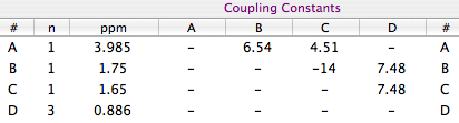In practice, we already know all the coupling constants, but the geminal one. We can set the initial value of the latter to -14 Hz, which is the common value for a geminal coupling.
Create a new spin system with the following parameters:

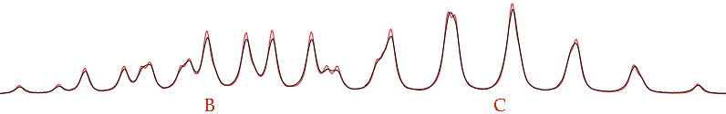
In our pictures, the experimental spectrum is black and the simulated one is red. It's a good idea if you too implement two contrasting colors. With the aid of the Overlay Manager, import the experimental spectrum as an overlay. After closing this manager, check the button at the left of “pop” (into the sidebar) and click on “assimilate”. Finally double click into the plot.

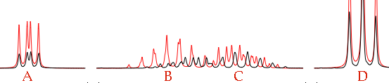
The first problem is to assign the coupling constants involving A. We don't know which is which. From the picture it seems that our first assignment was reversed. Try setting JAB = 4.51 and JAC = 6.54. Zoom into the central region (the outer regions are just OK, we can neglect them for a while). Move the letter C until the rightmost red peak covers the rightmost black peak. Move the letter B until the leftmost red peak covers the leftmost black peak.

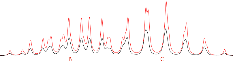
The name “total lineshape fitting” is a little misleading. It's normally better to fit limited regions (isolated multiplets or clusters of multiplets). Verify that only the region shown above (or a little more) is displayed into your window. Now check the following parameters: pop, B, C and all the Js. Give the command: Simulate/Fit to Overlay. At the end of the run, the result is:

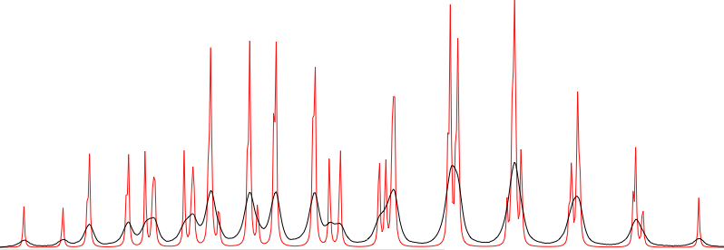
The fit is not perfect because we have not optimized the linewidths. In most of the cases, you are only interested into the Js. It doesn't matter if the simulated spectrum is not identical to the experimental one. Actually, it can be useful to move into the opposite direction. Try setting defW = 0.2 to see how many lines are the multiplets actually made of.

An IMPORTANT side effect of the fitting process is that the regions of the spectrum that are not shown are also REMOVED. To recreate the entire spectrum, it's simply necessary to click the button “refresh”.

You can keep playing with this spectrum. For example, trying to achieve a better fit with different linewidths for each nucleus (open the dialog “Simulate/Define” and uncheck the option “same width for all lines”). You can also try to fit the whole region from 0.8 to 4.1 ppm (although such a strategy is generally not advisable). The right strategy consists into fitting the easier multiplets first. In our case they were trivial first order multiplets, but in the general case they can require their own simulation. Continue fitting the clusters one by one, keeping immutable (i.e.: unchecked) those parameters that have already been optimized.